
Want to create a drop-down list in Excel? Here's a quick 5 step guide to creating drop-down lists
In today’s fast-paced world, whether you’re managing a business or simply trying to keep your household in order, staying organized is crucial. While there’s an abundance of apps and websites designed to aid in organization, my go-to solution has always been the reliable Microsoft Excel.
But Microsoft Excel is not just a relic from your parents’ desk jobs. When utilized effectively, it can serve as a powerful tool for business owners, professionals, or anyone needing to streamline tasks such as managing finances, schedules, or budgets. One handy feature within Excel is the ability to create drop-down lists, which can significantly simplify data entry and save valuable time.
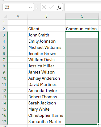
1. Select the cells where you want the drop-down list:
Identify the cells where you want to insert the drop-down lists. For instance, in a spreadsheet listing clients and their communication preferences, select the column where you’ll input communication preferences.
2. Select the Data Validation:
Click on “Data” and then select “Data Validation.” This will open a popup window
3. Choose list option:
In the Data Validation popup window, navigate to the “Allow” dropdown menu and select “List.”
4. Enter the list values of your drop-down list:
In the “Source” field of the popup, enter the items you want to include in the drop-down list, separated by commas. For example, if your options are “Call,” “Email,” “Text,” and “No Selection,” input them accordingly.
5. Save your drop-down list by clicking OK:
Click “OK” to save your drop-down list settings. Now, whenever you click on a cell within the specified range, a drop-down arrow will appear. Clicking on the arrow will reveal the list of options for selection.